Computational Modeling of the batemann equations
Author:
Philip Main
Last Updated:
12 years ago
License:
Creative Commons CC BY 4.0
Abstract:
Some Mphys work

\begin
Discover why over 25 million people worldwide trust Overleaf with their work.

\begin
Discover why over 25 million people worldwide trust Overleaf with their work.
\documentclass[a4paper]{article}

\usepackage[english]{babel}
\usepackage[utf8]{inputenc}
\usepackage{amsmath}
\usepackage{graphicx}
\usepackage[colorinlistoftodos]{todonotes}
\usepackage{caption}
\usepackage{subcaption}

\title{Computational Modeling of the \textsuperscript{238}U and \textsuperscript{232}Th Decay Chains}

\author{Philip Main}

\date{\today}

\begin{document}
\maketitle

\section{Introduction}
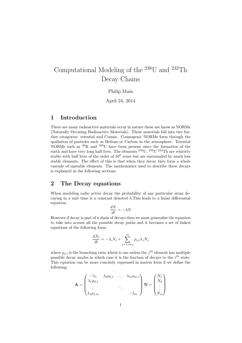
There are many radioactive materials occur in nature these are know as NORMs (Naturally Occuring Radioactive Materials). These materials fall into two further catagories: terestial and Cosmic. Cosmogenic NORMs form through the spallation of particles such as Helium or Carbon in the atmosphere. Terestial NORMs such as \textsuperscript{40}K and \textsuperscript{338}U have been present since the formation of the earth and have very long half lives. The elements \textsuperscript{238}U, \textsuperscript{235}U  \textsuperscript{232}Th are relativly stable with half lives of the order of $10^{9}$ years but are surrounded by much less stable elements. The effect of this is that when they decay they form a whole cascade of unstable elements. The mathematics used to describe these decays is explained in the following sections.

\section{The Decay equations}

When modeling radio active decay the probability of any particular atom decaying in a unit time is a constant denoted $\lambda$.This leads to a liniar differential equation:
$$ \frac{dN}{dt} = -\lambda N $$
However if decay is part of a chain of decays then we must generalise the equation to take into acount all the possible decay paths and it becomes a set of linked equations of the following form:
$$ \frac{dN_i}{dt} = -\lambda_i N_i + \sum_{j=1,i\neq j}^m \rho_{j,i} \lambda_j N_j $$
where $ \rho_{j,i} $ is the branching ratio which is one unless the $j^{th}$ element has multiple possible decay modes in which case it is the fraction of decays to the $i^{th}$ state. This equation can be more concisely expressed in matrix form if we define the following:

$$ \bf A = \begin{pmatrix}
    -\lambda_1 & \lambda_2 \rho_{2,1} & \ldots & \lambda_m \rho_{m,1} \\
    \lambda_1 \rho_{2,1} && \\
    \vdots && \ddots \\
    \lambda_1 \rho_{1,m} &&& -\lambda_m  \\
  \end{pmatrix}
  \bf N = \begin{pmatrix}
      N_1 \\
      N_2 \\
      \vdots \\
      N_m \\
    \end{pmatrix} $$
then we can express the set of linked equations as one matrix equation:
$$  \frac{d \bf N}{dt} = \bf A \bf N $$


\subsection{The Batemann Equation}
In the special case of an exit only decay chain then each radionuclide in the chain has only one parent and one child then the matrix $\bf A$ is zero exept for the diagonal and subdiagonal elements. The solution for this case is given by the batemann equations.

$$ N_m(t) = N(t=0) \prod_{i=1}^{m-1}\lambda_i \sum_{j=1}^m \frac{e^{-\lambda_j t}}{\prod_{k=1, k\neq j}^m (\lambda_k - \lambda_j)} $$
These equations are impractical to use on paper but easy to impliment on a computer. Using FORTRAN to implement these the some activity plots for \textsuperscript{238}U and \textsuperscript{232}Th were produced see fig.\ref{fig:activity}.

\begin{figure}
        \centering
        \begin{subfigure}[b]{0.50\textwidth}
                \includegraphics[width=\textwidth]{U-238.png}
        \end{subfigure}
        \begin{subfigure}[b]{0.50\textwidth}
                \includegraphics[width=\textwidth]{Th_232.png}
        \end{subfigure}
          \caption{Activity plots showing the elements of 4n+2 (\textsuperscript{238}U and decendents) and 4n (\textsuperscript{232}Th series)reaching secular equallibrium}\label{fig:activity}
\end{figure}

The 4n+2 decay chain contains many short lived isotopes; there are 14 orders of magnitude between the half lives of \textsuperscript{238}U and \textsuperscript{214}Po for this reason only the five longest lived radionuclide were included in the plot assuming that the shorter lived nuclide reach equallibrium almost instantanously with their longer lived parents. The nuclide in the \textsuperscript{232}Th decay series dont have such a varied range of half lives however the final nuclide in the chain \textsuperscript{208}Pb has two parents so the batemann equations are not ideal for solving this problem. The next program I wrote was a integrated the matrix decay equation with using the Runge Kutta method. Despite having a local truncation error $\mathcal{O}(h^5)$ the variations in half life doesn't allow for a sensible time step to be set for the whole chain although this method would be useful for sections of the chain.


\subsection {The Matrix Aproach}
There is a more general way of solving the matrix decay equation which takes the following form:

$$ {\bf N = V \Lambda V^{-1} N(}t=0) $$
where
$$ \bf V = \begin{pmatrix}
    \upsilon_1 \\
    \upsilon_2 \\
    \vdots \\
    \upsilon_m \\
    \end{pmatrix}
   \Lambda = \begin{pmatrix}
     e^{-\mu_1 t} &&&& \\
     & e^{-\mu_2 t}  \\
     && \ddots \\
     &&& e^{-\mu_m t}
     \end{pmatrix}
  $$
and $\upsilon$, $\mu$ denote the eigenvectors and eigenvalues of matrix {\bf A}. This solution requires $\upsilon$ and $\mu$ values to be solved for each decay series. To do this routines to find the eigenvalues of the system, the matrix $\Lambda$ and the inverse of $\Lambda$ from the LAPack (linear algebra package) library were integrated into a FORTRAN program. The halflife and branching ratio data from the 4n decay series was used to produce fig.\ref{fig:activity2}. This chain branches at \textsuperscript{212}Bi this can is seen by the activities of \textsuperscript{212}Po and \textsuperscript{208}Tl which are lower in the equallibrium state than the other members in the chain. This because the sum of their activities is equal to the activity of \textsuperscript{212}Bi at this point. In both of the decay chains which I used to test my programs secular equallibrium is reached very quickly, the 4n chain takes about $10^{-18}$ of the half life of \textsuperscript{232}Th and about $10^{-3}$ of \textsuperscript{238}U when starting from a pure source.

\begin{figure}
\centering
\includegraphics[width=\textwidth]{4n.png}
\caption{plot of 4n sereis using the matrix aproach taking branching into acount}
\label{fig:activity2}
\end{figure}


\end{document}